Harnessing KNN & Neural Nets to Assess Default Risk for Unbanked Loan Applicants
Introduction
Lending money is a profitable enterprise but only if you’re loaning to people that pay back their loans. Therefore, it is very important for banks and companies to be able to assess beforehand whether or not a person is likely to repay a loan. Many criteria have been considered over the years in attempts to gauge the responsibility of a borrower including but not limited to the borrower’s previous loan history, the area in which they are living, and how long it has been since they changed phone numbers. One of the key metrics used in the credit history, a measure of how you have behaved with previous loans calculated from how much you borrow, how often you make late payments, and how often you default. Most lending entities today prioritize credit history as their metric of choice when considering loan applications and often will not loan to applicants who cannot present a satisfactory credit history.
However, this leads to a problem for both the loaners and the borrowers: the borrowers cannot get the capital they might need without submitting to terrible loan deals and the loaners leave a large population of customers untapped. By analyzing nonstandard metrics other than credit history to predict the trustworthiness of a borrower, this analysis seeks to bridge this gap. An accurate classification model could provide the loan entities with some assurance that their loans will be repaid and that, with less risk, they would be more willing to loan to this non borrowing population, benefiting everyone.
To address this issue, an initial exploratory factor analysis (EFA) is conducted, in which I attempt to recover latent variables relating to clients’ trustworthiness. The hope is that such observations will be informative to future attempts at classification and in the compiling of other data sets. In other words, by finding which variables in our data set are most informative, companies and researchers can prioritize them both at the data collection stage and at the evaluation stage.
After this, a k-nearest neighbors classifier is applied to the data to form a predictive model. This model, if accurate, would be a major deliverable of the project and ready for use by loan entities. At the very least this attempt at classification will inform us as to whether or not the quantitative variables being collected and used are informative to the question of interest.
A logistic neural net is also applied (with the same rationale as the k-nearest neighbor model). It’s chosen because we are interested in seeing whether we can do a better job in predicting whether or not a client will default on a loan. A neural net is a platform for many machine learning techniques. A system of neuron nodes are set up each with a different random weights and connected to a random selection of the input variables. The process runs on the training set to classify the data and then adjusts the weights of its neurons based on the most erroneous cases, repeating until the weights of the neurons are no longer adjusting or until some other specified cutoff point is reached. By using both of these classification methods, we will compare the two models and either confirm the accuracy or our predictions or indicate more work is needed on one model or the other.
Data
The data used comes from the Home Credit Group which is interested in giving loans to clients that have no credit history. As such, other metrics must be used and the challenge of this dataset is evaluating a borrower’s likelihood of repaying from these other criteria. The 307511 observation dataset of loans contains 122 alternative variables and is not terribly tidy. Some extra work is needed before working with the dataset.
Firstly, a uniform random sample of the dataset is taken to cut it down to 10,000 observations. We then pare down the dataset’s variables by eliminating any with less than 90% complete observations. This leaves us with 66 variables, most of them indicator flags of whether an applicant met this or that criteria. Upon some further trimming, we decide to use the following nine quantitative variables:
-
Target: binary indicator of default, 0 is no default, 1 is default.
-
Income: annual income of the borrower
-
Loan amount: the dollar amount of the requested loan
-
Loan annuity: how much collateral the borrower could present
-
Region Population: the normalized level of population for that area
-
Client Age: age in years
-
Length of Employment: negative values indicate unemployment
-
Number of Family Members
-
Days Since Last Phone Change
Extraction
We query an SQLite database to obtain client information using the DBI package. The dbConnect() function is used to create a database connection. Invoking it returns an object that can be used to communicate with the database management system (DBMS), providing access to dynamic queries, results and management sessions.
##   Target Income  Amount Annuity      Pop    Age    Emp Fam Phone
## 1      0 157500  288873 14805.0 0.022625 -10676  -1190   2    -2
## 2      0 207000  781920 34573.5 0.046220 -21762 365243   1  -882
## 3      0 103500  161730 11385.0 0.024610 -17623  -1636   3 -2293
## 4      0 405000 1800000 47614.5 0.010006 -13362   -232   4  -309
## 5      0 157500  545040 25537.5 0.025164 -13115  -6211   1     0
## 6      0 157500  314055 17167.5 0.003122 -16330  -1971   3  -808
The table above shows the first six client entries after obtaining the 9 variables of interest.
Exploratory Analysis
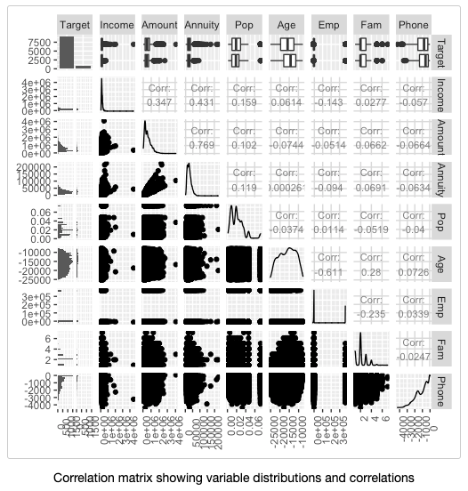
A correlation matrix is constructed from the quantitative variables to get a closer look at correlation values as well as the distributions of the variables in our dataset. Most of the correlations were weak. The only strong correlation observed was between loan annuity and loan amount which makes sense since we would expect the bank to be willing to loan more money if more collateral is presented. Most of the variables are right skewed. It is also interesting to see the presence of multiple distinct peaks among the different variable distributions.

Methods
Experiments
In addition to being listed on this report, the experiments conducted in this study are shared and maintained on Tableau Public. Feel free to check out my published worksheet below!

Factor Analysis
A Factor Analysis is more appropriate in this analysis than Principal Components Analysis because we are interested in seeing which latent indicators of trustworthiness / ability to pay back loans can be recovered from a set of manifest variables. A Maximum Likelihood Approach is used to determine, through repeated hypothesis testing, which number of factors is most appropriate.
Classification
K Nearest Neighbors:
- KNN classifiers with 10 values of k (1-10) are fitted and represented on plots showing the apparent and estimated error rates for the various values of k. An 80% ~ 20% holdout sample approach is used here to obtain the respective train and test sets.
Neural Nets:
- The second classification method used was neural nets. Neural nets are composed of layers of weighted neurons that pass on 0 or 1 depending on whether the weighted sums of their inputs exceed their activation potential. The system is modeled after the function of the neurons in the human brain. By working on the training set iteratively, the weights of the neurons can be refined based on the misclassifications until all training samples are classified (or, to reduce over fitting, until a certain number of iterations have been reached). By layering these sets of neurons and having the outputs of one layer be fed into the next, you can do this weight-refining approach several times and achieve accuracy in complex classifications far beyond the scope of regression, as evidenced by their use in photo analysis, voice identification, and of course in our own heads.
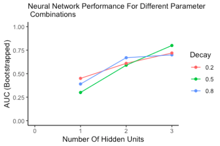
In this case, a holdout sample approach was used to evaluate the sufficiency of the neural network model. The proportions chosen were 75% ~ 25% for the train and test set respectively. The caret package is used to find the best parameters to use for this classifier. To kick start the process, we set up a grid of tuning parameters for the model, fitted each and calculated a bootstrapped AUC (Area under ROC curve) score for every hyper parameter combination. The values with the biggest AUC are chosen for the neural network. The preferred evaluation metric is AER and estimated TER, but the only available ones are: sensitivity, specificity, area under the ROC and AUC. It is worth noting that all available predictors are used to fit the model. The final parameters chosen are: three interconnected neuron layers with a decay rate of 0.5 (factor by which each weight is multiplied by after each update.)1. The weighted inputs and bias are summed to form the net input to the next layer. The inputs are mapped from layer to layer then finally fed into a sigmoid function that outputs the desired probability that a client will default.
Results
Factor Analysis
Five possible factor solutions are examined to find one with the most compelling interpretation. Although the p-values yielded from the maximum likelihood evaluation of the five factor solution suggested that none of them could adequately account for the variations in the data, the factors in the five factor model satisfy the principles of Thurstone’s simple structure. The first factor in this model loads highly on credit and annuity thus it could be labelled non-Income assets. The second one is a contrast between age and duration of employment. The third is dominated by continuous family members therefore it could be seen as a measure of client mobility. The fourth reflects income whereas the fifth seems like a weighted average.
#Call:
factanal(x = train_sample, factors = 5)
Uniquenesses:
| Income Amount | Credit Amount | Annuity | Region Pop | Days Birth | Days Employed | Days Registration | Days ID Publish | Fam Members | Last Phone Change |
|---|---|---|---|---|---|---|---|---|---|
| 0.394 | 0.005 | 0.350 | 0.947 | 0.342 | 0.165 | 0.760 | 0.782 | 0.675 | 0.929 |
Loadings:
| Factor 1 | Factor 2 | Factor 3 | Factor 4 | Factor 5 | |
|---|---|---|---|---|---|
| Income Amount | 0.218 | 0.106 | 0.735 | ||
| Credit Amount | 0.979 | 0.175 | |||
| Annuity | 0.716 | 0.356 | |||
| Region Pop | 0.206 | ||||
| Days Birth | 0.600 | 0.496 | 0.219 | ||
| Days Employed | -0.841 | -0.300 | 0.185 | ||
| Days Registration | 0.179 | 0.377 | 0.253 | ||
| Days ID Publish | 0.392 | 0.248 | |||
| Fam Members | 0.546 | -0.116 | |||
| Last Phone Change | 0.258 |
| Factor 1 | Factor 2 | Factor 3 | Factor 4 | Factor 5 | |
|---|---|---|---|---|---|
| SS loadings | 1.532 | 1.263 | 0.802 | 0.753 | 0.301 |
| Proportion Var | 0.153 | 0.126 | 0.080 | 0.075 | 0.030 |
| Cumulative Var | 0.153 | 0.280 | 0.360 | 0.435 | 0.465 |
K Nearest Neighbors
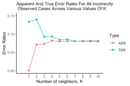
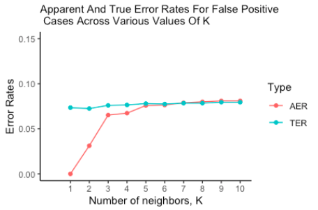
Figure1 is the graph of the AER and TER for the KNN runs on values of K from 1:10. Larger values of k perform fairly well. Additionally, we see a convergence toward a 0.08 error rate in both the AER and the TER. However, due to the nature of our data, we shouldn’t treat all error rates equally. From the viewpoint of the company, mistakenly classifying a paying borrower as nonpaying is less harmful than classifying a nonpaying borrower as paying. In other words, a false positive from our classifier means we give a loan that is not paid back. Let’s consider the error rate of only these harmful errors in Figure2.
We can see in Figure2 that the AER behaves essentially identically to the run with both error rates while the TER is markedly different in the beginning but then both continue to approach 0.08. This suggests that, as we increase k, we eliminate the Type I errors of our model on new data. Unfortunately the harmful Type II error rate is not eliminated and remains at 0.08. This means that we should expect 8% of the applicants given the go-ahead by our model to actually not repay their loans. On the upside however, if our model indicates an applicant cannot be trusted, it is almost always correct.


Neural Networks
The results obtained from the grid search process show that the prediction accuracy increases as a function of the number of units in the hidden layer of the neural network. There is also a discernible improvement in model quality for moderate weight decay values. The estimated true error rate was 8.64% and the apparent error rate was 8.87%. Both of these error rates are based on a majority class prediction.

Conclusions
From the results obtained from this analysis, we can reasonably recommend the adaptation of a KNN classifier due to its robust performance in predicting default risk. Although a neural network performs similarly, it proved to be an extremely slow learner that takes long to run. More data and resamples would have been brought in given more time and resources to see whether the observed issues with multivariate normality can be fixed. It is also important to note that the scope of inference from the methods used in this analysis are only applicable to individuals with similar histories to those in this study.
Citations
- Brownlee, Jason. “Tuning Machine Learning Models Using the Caret R Package.” Machine Learning Mastery, 22 Sept. 2016, www.machinelearningmastery.com/tuning-machine-learning-models-using-the-caret-r-package/.
- Portilla, Jose. “KDnuggets.” KDnuggets Analytics Big Data Data Mining and Data Science, 2016, www.kdnuggets.com/2016/08/begineers-guide-neural-networks-r.html.
- “Weight Decay in Neural Networks.” Metacademy, metacademy.org/graphs/concepts/weight_decay_neural_networks.
- R documentation caret package
- Multivariate Analysis With R
- Wickham, H. (n.d.). R Database Interface (DBI 1.1.0). Retrieved December 11, 2020, from https://dbi.r-dbi.org/