Forecasting Methods for Modelling Changing Variance in Time Series
Abstract
This project is based on exploring ARCH /GARCH methods and their application in modelling the changing variance of time in predicting stock prices. The data used in this study is obtained from the S&P 500 index, which is a measure that estimates the performance of 500 companies listed in the United States Stock exchange market. The data used includes daily data spanning the years 2013 - 2018.
Introduction - ARIMA models
The first phase of this analysis begins with the exploration of an ARIMA, where ARIMA stands for Auto Regressive Moving Average models. They consist of two components; the Autoregressive Component and the Moving Average Component and are denoted as ARIMA(p,d,q), with p representing the number of autoregressive terms, d the number of differencing and q the number of Moving Average terms. The second phase involves the checking of model residuals (to look for volatile clusters) followed by an eventual transition to ARCH/GARCH.
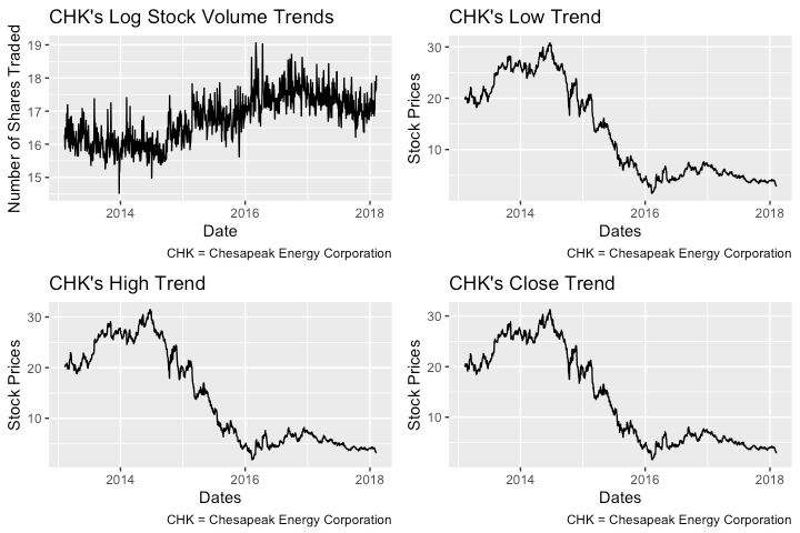
Before we begin any model fitting, we make the line graphs shown below. This step is meant as an initial exploration aimed at showing the trends in volume and price of Chesapeake Energy Corporation’s stocks. All the plots below are similar because they show that the volume, opening, high and low values exhibited high volatility. Volatility in a time series refers to the phenomenon where the conditional variance of a time series varies over time (Cryer and Chan, 2008). Stock volume seems more volatile than low, high and close prices, as can be seen from the more sudden irregular shifts in trends with time.
The data wrangling required before fitting the model/ checking conditions is minimal. It begins by decomposing Chesapeake monthly data time series into seasonal, trend and irregular components, then moves on to the removal of seasonal components to create a seasonally adjusted component.
Model Conditons
Before fitting an ARIMA time series model, we need to make sure that it is free of trends and non seasonal behavior. We also check to make sure that the time series has a constant mean and variance. If variation in trends is present, we difference in order to get rid of those trends and prepare the data for model fitting. After all these checks are performed, we run the Augmented Dickey Fuller test to make sure that stationarity is satisfied:
The hypothesis test to check whether our data is stationary is as follows:
$H_0$: Chesapeake time series is not stationary.
$H_A$: Chesapeake time series is stationary.
Our test yields a statistic of −3.5423 and a p value of 0.03823. We therefore reject the null as there is strong evidence of stationarity in the data, and proceed to the model fitting phase.
#adf test checks whether ts is stationary or not (data condition)
adf.test(CHK_deseasonal_value, alternative = "stationary")
##
##  Augmented Dickey-Fuller Test
##
## data:  CHK_deseasonal_value
## Dickey-Fuller = -3.5423, Lag order = 10, p-value = 0.03823
## alternative hypothesis: stationary
Model Fitting
Here, we use the Auto.arima() function to help obtain model parameters using a stepwise model fitting procedure. This model selection procedure selects the model with the lowest AIC value. The p, d, q parameters of the model will be selected from the model with the lowest score. We start with a maximum order of 6 for all parameters and iterate through different combinations to find one that produces the model with the lowest AIC score:
#auto fits arima model
CHK_fit = auto.arima(CHK_deseasonal_value, max.order = 6)
CHK_fit
## Series: CHK_deseasonal_value
## ARIMA(4,1,3)
##
## Coefficients:
##          ar1     ar2     ar3      ar4     ma1      ma2      ma3
##       0.2097  0.3550  0.6572  -0.4885  0.2163  -0.3094  -0.7638
## s.e.  0.0449  0.0418  0.0359   0.0263  0.0468   0.0452   0.0373
##
## sigma^2 estimated as 1.864e+12:  log likelihood=-19460.3
## AIC=38936.59   AICc=38936.71   BIC=38977.65
The model chosen from our selection procedure has 4 Autoregressive Terms i.e AR(4), a differencing of degree 1 and 3 moving average terms i.e MA(3). The fitted model from the parameters obtained above can be expressed as :
$$\hat{Y}_{t} = 0.2097 Y_{t-1}+0.3550 Y_{t-2}+0.6572 Y_{t-3}-0.4885 Y_{t-4}+0.2163 e_{t-1}-0.3094 e_{t-2}-0.7638 e_{t-3}+\epsilon$$
The equation above is a linear combination of terms. The Y’s correspond to recent stock volume values up until the $(t-4)^{th}$ time step while the $e$’s correspond to the errors of the lags at the denoted, corresponding time steps.
In the next section we shall examine sample partial autocorrelation (PACF) and sample autocorrelation plots (ACF) to validate our choices of the p, d and q orders chosen for our ARIMA model by the stepwise model selection procedure.
Model Diagnostics
Before settling down on the model obtained from the previous section, we examine the auto correlation of residuals to make sure our model is free of auto correlations. This is necessary because it helps us establish whether the noise terms in the model are independent from each other:
ggtsdisplay(residuals(CHK_fit), plot.type = "partial",
            main = "ARIMA (4, 1, 3) Diagnostic plots")
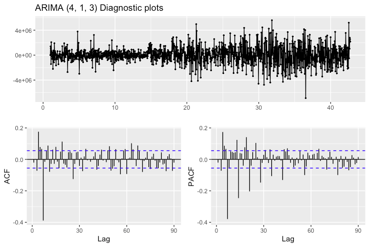
A quick examination of the ACF plot reveals the existence of excessive correlations in the residuals at lags 3 and 6. Furthermore, the lag patterns in the PACF are quite similar to those in the ACF plot, suggesting the existence of autocorrelation. This problem in distribution of error terms also manifests itself in the residuals, and can be seen from the unequal variation of error terms across the range of values in the residual plot.
In order to confirm the findings from the diagnostic plots above, we conduct an official hypothesis test for model fit using the Ljung - Box test to see whether the error terms in the model are independently and identically distributed (i.i.d).
The Ljung Box test statistic is given by (Glen, 2018): $$Q_* = n(n+2) \sum_{k=1}^{m} \frac{r_{k}^{2}}{n-k}$$ where n is the size of the time series and r the residual correlation at the $k^{th}$ lag . $Q_*$ has a chi-square distribution with k-p-q degrees of freedom (Cryer and Chan, 2008). The official hypothesis for the test are as follows:
$H_0$ : The model error terms are uncorrelated
$H_A$ : The model error terms are correlated
Box.test(residuals(CHK_fit), lag = 90, fitdf = 83, type = 'Ljung-Box')
##
##  Box-Ljung test
##
## data:  residuals(CHK_fit)
## X-squared = 541, df = 7, p-value < 2.2e-16
Running the test yields a p value of 2.2e-16. We have sufficient evidence to reject the null, as there is strong evidence that the model assumption of independence of error terms has been violated. In the next section we attempt to find the remedy to this problem by exploring methods that model the changing variance in time series.
ARCH/ GARCH models
Introduction
In the previous chapter we tried fitting and assessing the feasibility of an ARIMA model on Chesapeake Energy Corporation’s stock data. The fitted model wasn’t appropriate because the model’s error terms were not independent and identically distributed. In addition, cluster volatility seemed to be a huge issue as observed from the heteroschedastic nature of modeled stock volume returns.
In this section we will use autoregressive conditional heteroschedastic models in an attempt to adequately capture and account for the heteroscedasticity observed in the ARIMA model. ARCH/GARCH are time series models used to model processes where volatility is high in provided data (Cryer and Chan, 2008). Cases involving stock market data are usually prone to unpredictable changes, and are best modeled using methods that model the variability of future values based on present and past provided trends in observed returns.
1. ARCH models
ARCH models are denoted ARCH(p), where p represents the order of the model. According to Cryer and Chan (2008) an ARCH(1) process modelling the return of a time series r takes the form $r_{t}=\sigma_{t | t-1} \varepsilon_{t}$ where $\varepsilon_{t}$ is a series of independent and identically distributed random variables with a mean of zero and standard deviation of 1. The quantity $\sigma_{t | t-1}$ models the conditional variance, $\sigma_{t | t-1}^{2}$, of the return $r_{t}$, and is given by $\sigma_{t | t-1}^{2}=\omega+\alpha r_{t-1}^{2}$. The variance of the current return is based on conditioning upon returns until the ${(t-1)}^{th}$ time step. The quantities $\omega$ and $\alpha$ represent the ARCH model intercept and coefficient respectively.
The diagram below represents a sample ARCH(1) process simulated with $\omega$ = 0.1 and $\alpha$ = 0.5 as the chosen model parameters.
set.seed(85)
garch01.sim = garch.sim(alpha=c(.1,.5),n=400)
sim_data <- data.frame(seq(1,400),garch01.sim )
arch.plt <- ggplot(sim_data, aes(x = seq.1..400., y = garch01.sim )) + geom_line() +
  xlab("Time Step") + ylab("Return at Time Step t") +
  ggtitle("Simulated ARCH(1) process")
ggplotly(arch.plt)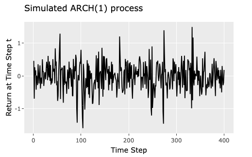
2. GARCH models
The ARCH model introduced in the previous section models future returns by conditioning the value of the variance at time t to the previous time step alone i.e $\sigma_{t | t-1}^{2}=\omega+\alpha r_{t-1}^{2}$. Bollerslev’s (1986) approach encourages the backward extension of this conditioning process up until the $q^{th}$ time step as well as the introduction of p lags to the conditional variance (Cryer and Chan, 2008). This resulting model becomes a Generalized Autoregressive Conditional Heteroscedasticity (GARCH) process, and is denoted as GARCH(p,q). The return from this new proposed model takes the same form as ARCH’s $r_{t}=\sigma_{t | t-1} \varepsilon_{t}$. However, the conditional variance $\sigma^2_{t | t-1}$ modeled by the quantity $\sigma_{t | t-1}$ now becomes : $$\begin{aligned}
\sigma_{t | t-1}^{2}=\omega+\beta_{1} \sigma_{t-1 | t-2}^{2}+\cdots+& \beta_{p} \sigma_{t-p | t-p-1}^{2}+\alpha_{1} r_{t-1}^{2}+\alpha_{2} r_{t-2}^{2}+\cdots+\alpha_{q} r_{t-q}^{2}
\end{aligned}$$
The $\beta$ coefficients in the model are used to assign weights to the lags of the conditioned variance values.
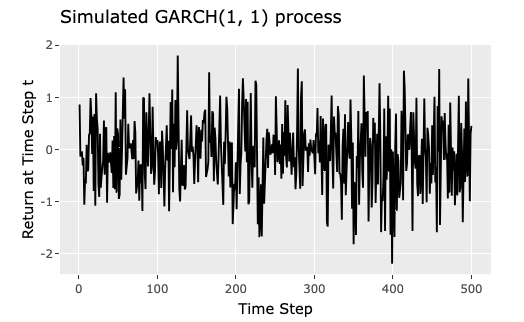
The plot below (Cryer and Chan, 2008) illustrates an example of a simulated GARCH(1,1) process with parameter values $$\omega=0.02, \alpha=0.05, \text { and } \beta = 0.9$$
The parameters $\omega, \beta, \alpha$ in GARCH and $\omega, \alpha$ in ARCH are constrained to $>0$, since the conditional variances have to be positive.
Estimation of GARCH model coefficents
GARCH model coefficients are fit using the Maximum Likelihood Approach. The estimation process used to obtain the likelihood estimates for $\omega, \beta, \alpha$ is based on recursively iterating through the log likelihood function modelling the GARCH coefficient estimates. The log likelihood function we aim to maximize is defined as (Cryer and Chan, 2008):
$$L(\omega, \alpha, \beta)=-\frac{n}{2} \log (2 \pi)-\frac{1}{2} \sum_{i=1}^{n}\left\{\log \left(\sigma_{t-1 | t-2}^{2}\right)+r_{t}^{2} / \sigma_{t | t-1}^{2}\right\}$$Model Fitting
Below, we try fitting an appropriate GARCH model using the ugarchfit() function from the rugarch package. The package computes the model estimates using the maximum likelihood function specified in the previous section.
We will explore different GARCH orders, with the aim of finding the model that best fits the data. The orders we will try are arbitrarily chosen as GARCH(1,1), GARCH(2,2)and GARCH(3,3):
Model Diagnostics
The GARCH(1,1) model seems like the most appropriate here since all but one of it’s model coefficients are significant. Furthermore, it has the lowest AIC of all the models explored.
Before we accept the model we found in the previous section we need to make sure that assumptions have been met for the ARCH(1,1) model. The squared residuals need to be serially uncorrelated and the error terms should be normally distributed:
#QQplot to check for normality
qqnorm(residuals(fit_mod1)); qqline(residuals(fit_mod1))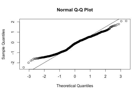
#Sample acf and pacf plots to check iid assumption
ggtsdisplay(residuals(fit_mod1), plot.type = "partial",
            main = "Chesapeak Energy Corporation's GARCH (1, 1) Diagnostic plots")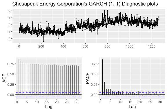
From the diagnostic plots made above, we see a major problem with normality, as most of the points on the qqplot veer off the line. In addition, there seems to be major issues with independence, as can be seen from the significant lags in residuals from the autocorrelation plots.
Results
From the model diagnostics we ran in the previous section, we discovered major issues with normality and independence in error terms. We might want to explore more model parameters to see whether we can find a model that improves upon what we currently have. For now, we will proceed with extreme caution and use the GARCH(1,1) model to make some predictions.
Below, we extract the coefficients from the chosen GARCH(1,1) model.
#Extract coefficients
fit_mod1@fit$matcoef
## Estimate Std. Error t value Pr(>|t|)
## mu 16.96828513 0.03046360 557.001998 0.000000e+00
## omega 0.04592897 0.01059138 4.336448 1.448039e-05
## alpha1 0.40407479 0.05760516 7.014559 2.306821e-12
## beta1 0.51414297 0.06573577 7.821358 5.329071e-15The return at time t as given by our model is going to be given by (Boudt, 2020) : $$R_{t} = 16.97 +e_{t}$$ where the $e_{t}$ is a normally distributed random variable with a mean of 0 and variance of $\widehat{\sigma}_{t}^{2}$ i.e $e_{t} \sim N\left(0, \widehat{\sigma}_{t}^{2}\right)$. The variance modelling return volatility at the $t^{th}$ time step in our fitted model is going to be $\widehat{\sigma}_{t}^{2}=0.05+0.40 e_{t-1}^{2}+0.51 \widehat{\sigma}_{t-1}^{2}$
The ugarchroll() function is used to obtain estimates for the last four dates in the data set. The test data that is used is the most recent week’s returns in stock volume. The log volume residuals obtained after this process are printed down below :
#Forecasting using the ugarchforecast function
preds = ugarchforecast(fit_mod1, n.ahead = 1, data = CHK[1255:1259, ,drop = F][,6])
preds = ugarchroll(spec = spec_mod1 , data = log(CHK_ts) , n.start = 1255 , refit.every = 2 , refit.window = 'moving')
References
- Cryer, J. D., & Chan, K.-sik. (2008). Time series analysis with applications in R. New York: Springer.
- Nugent, C. (n.d.). S&P 500 stock data. Retrieved from https://www.kaggle.com/camnugent/sandp500.
- Boudt, K. (n.d.). GARCH Models in R. Retrieved from https://www.datacamp.com/courses/garch-models-in-r.
- Trapletti, A., & Hornik, K. (n.d.). Package ‘tseries.’ Retrieved from https://cran.r-project.org/web/packages/tseries/tseries.pdf
- Ghalanos, A., & Kley, T. (n.d.). Package ‘rugarch.’ Retrieved from https://cran.r-project.org/web/packages/rugarch/rugarch.pdf
- Glen, S. (2018, September 11). Ljung Box Test: Definition. Retrieved from https://www.statisticshowto.datasciencecentral.com/ljung-box-test/
- Bollerslev, T. (1986). Generalized autoregressive conditional heteroskedasticity. Journal of Econometrics, 31(3), 307–327. doi: 10.1016/0304-4076(86)90063-1